Multi-threaded solving

1. Multi-threaded solving

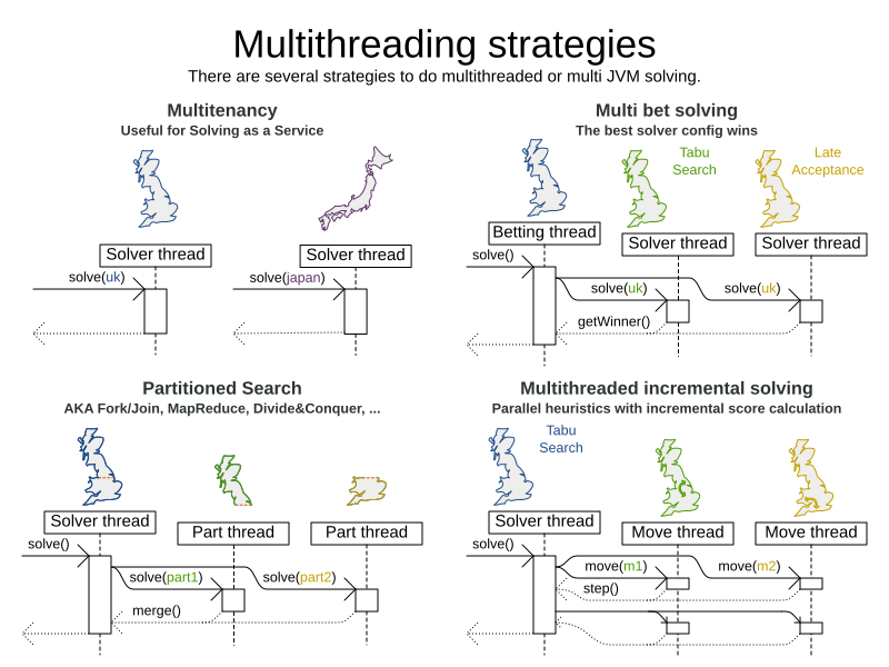
There are several ways of running the solver in parallel:

Multi-threaded incremental solving: Solve 1 dataset with multiple threads without sacrificing incremental score calculation.
Partitioned search: Split 1 dataset in multiple parts and solve them independently.
Multi bet solving: solve 1 dataset with multiple, isolated solvers and take the best result.
- Not recommended: This is a marginal gain for a high cost of hardware resources.
- Use the Benchmarker during development to determine the algorithm that is the most appropriate on average.
Multitenancy: solve different datasets in parallel.
- The SolverManager can help with this.

1.1. Multi-threaded incremental solving

This feature is exclusive to Timefold Solver Enterprise Edition.

With this feature, the solver can run significantly faster, getting you the right solution earlier. It has been designed to speed up the solver in cases where move evaluation is the bottleneck. This typically happens when the constraints are computationally expensive, or when the dataset is large.

The sweet spot for this feature is when the move evaluation speed is up to 10 thousand per second. In this case, we have observed the algorithm to scale linearly with the number of move threads. Every additional move thread will bring a speedup, albeit with diminishing returns.
For move evaluation speeds on the order of 100 thousand per second, the algorithm no longer scales linearly, but using 4 to 8 move threads may still be beneficial.
For even higher move evaluation speeds, the feature does not bring any benefit. At these speeds, move evaluation is no longer the bottleneck. If the solver continues to underperform, perhaps you’re suffering from score traps or you may benefit from custom moves to help the solver escape local optima.

These guidelines are strongly dependent on move selector configuration, size of the dataset and performance of individual constraints. We recommend you benchmark your use case to determine the optimal number of move threads for your problem.

1.1.1. Enabling multi-threaded incremental solving

Enable multi-threaded incremental solving by adding a @PlanningId annotation on every planning entity class and planning value class. Then configure a moveThreadCount:

Service / Quarkus
Spring
Java
XML

Add the following to your application.properties:

quarkus.timefold.solver.move-thread-count=AUTO

Add the following to your application.properties:

timefold.solver.move-thread-count=AUTO

Use the SolverConfig class:

SolverConfig solverConfig = new SolverConfig()
    ...
    .withMoveThreadCount("AUTO");

Add the following to your solverConfig.xml:

<solver xmlns="https://timefold.ai/xsd/solver" xmlns:xsi="http://www.w3.org/2001/XMLSchema-instance"
xsi:schemaLocation="https://timefold.ai/xsd/solver https://timefold.ai/xsd/solver/solver.xsd">

    ...
    <moveThreadCount>AUTO</moveThreadCount>
    ...

</solver>

Setting moveThreadCount to AUTO allows Timefold Solver to decide how many move threads to run in parallel. This formula is based on experience and does not hog all CPU cores on a multi-core machine.

A moveThreadCount of 4 saturates almost 5 CPU cores. The 4 move threads fill up 4 CPU cores completely and the solver thread uses most of another CPU core.

The following moveThreadCounts are supported:

NONE (default): Don’t run any move threads. Use the single threaded code.
AUTO: Let Timefold Solver decide how many move threads to run in parallel. On machines or containers with little or no CPUs, this falls back to the single threaded code.
Static number: The number of move threads to run in parallel.

It is counter-effective to set a moveThreadCount that is higher than the number of available CPU cores, as that will slow down the move evaluation speed.

In cloud environments where resource use is billed by the hour, consider the trade-off between cost of the extra CPU cores needed and the time saved. Compute nodes with higher CPU core counts are typically more expensive to run and therefore you may end up paying more for the same result, even though the actual compute time needed will be less.

Multi-threaded solving is still reproducible, as long as the resolved moveThreadCount is stable. A run of the same solver configuration on 2 machines with a different number of CPUs, is still reproducible, unless the moveThreadCount is set to AUTO or a function of availableProcessorCount.

1.1.2. Advanced configuration

There are additional parameters you can supply to your solverConfig.xml:

<solver xmlns="https://timefold.ai/xsd/solver" xmlns:xsi="http://www.w3.org/2001/XMLSchema-instance"
    xsi:schemaLocation="https://timefold.ai/xsd/solver https://timefold.ai/xsd/solver/solver.xsd">
  <moveThreadCount>4</moveThreadCount>
  <threadFactoryClass>...MyAppServerThreadFactory</threadFactoryClass>
  ...
</solver>

To run in an environment that doesn’t like arbitrary thread creation, use threadFactoryClass to plug in a custom thread factory.

1.2. Partitioned search

This feature is exclusive to Timefold Solver Enterprise Edition.

1.2.1. Algorithm description

It is often more efficient to partition large data sets (usually above 5000 planning entities) into smaller pieces and solve them separately. Partition Search is multi-threaded, so it provides a performance boost on multi-core machines due to higher CPU utilization. Additionally, even when only using one CPU, it finds an initial solution faster, because the search space sum of a partitioned Construction Heuristic is far less than its non-partitioned variant.

However, partitioning does lead to suboptimal results, even if the pieces are solved optimally, as shown below:

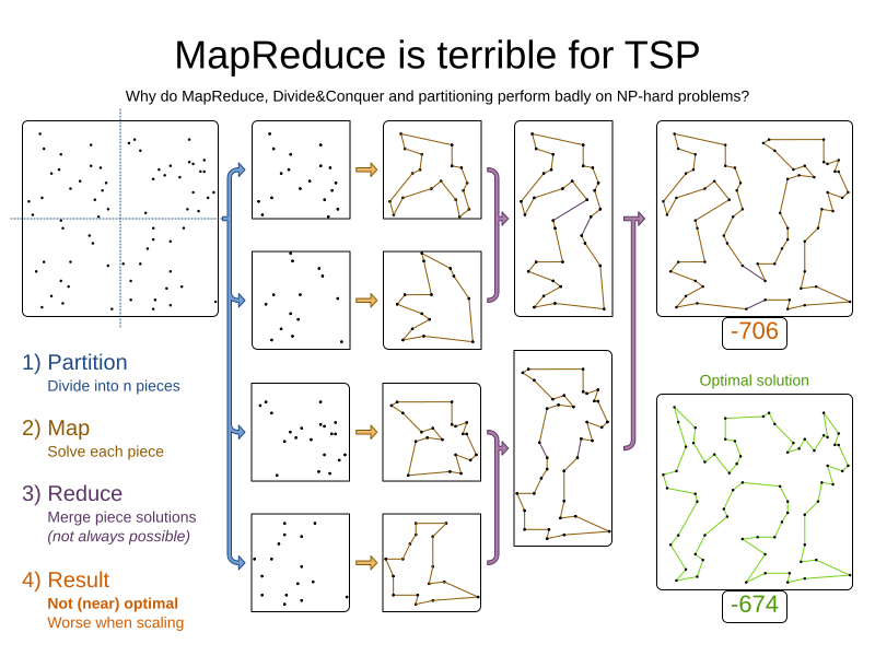
It effectively trades a short term gain in solution quality for long term loss. One way to compensate for this loss, is to run a non-partitioned Local Search after the Partitioned Search phase.

Not all use cases can be partitioned. Partitioning only works for use cases where the planning entities and value ranges can be split into n partitions, without any of the constraints crossing boundaries between partitions.

1.2.2. Configuration

Simplest configuration:

  <partitionedSearch>
    <solutionPartitionerClass>...MyPartitioner</solutionPartitionerClass>
  </partitionedSearch>

Also add a @PlanningId annotation on every planning entity class and planning value class. There are several ways to partition a solution.

Advanced configuration:

  <partitionedSearch>
    ...
    <solutionPartitionerClass>...MyPartitioner</solutionPartitionerClass>
    <runnablePartThreadLimit>4</runnablePartThreadLimit>

    <constructionHeuristic>...</constructionHeuristic>
    <localSearch>...</localSearch>
  </partitionedSearch>

The runnablePartThreadLimit allows limiting CPU usage to avoid hanging your machine, see below.

To run in an environment that doesn’t like arbitrary thread creation, plug in a custom thread factory.

A logging level of debug or trace causes congestion in multi-threaded Partitioned Search and slows down the move evaluation speed.

Just like a <solver> element, the <partitionedSearch> element can contain one or more phases. Each of those phases will be run on each partition.

A common configuration is to first run a Partitioned Search phase (which includes a Construction Heuristic and a Local Search) followed by a non-partitioned Local Search phase:

  <partitionedSearch>
    <solutionPartitionerClass>...MyPartitioner</solutionPartitionerClass>

    <constructionHeuristic/>
    <localSearch>
      <termination>
        <diminishedReturns />
      </termination>
    </localSearch>
  </partitionedSearch>
  <localSearch/>

1.2.3. Partitioning a solution

Custom `SolutionPartitioner`

To use a custom SolutionPartitioner, configure one on the Partitioned Search phase:

  <partitionedSearch>
    <solutionPartitionerClass>...MyPartitioner</solutionPartitionerClass>
  </partitionedSearch>

Implement the SolutionPartitioner interface:

public interface SolutionPartitioner<Solution_> {

    List<Solution_> splitWorkingSolution(Solution_ workingSolution, Integer runnablePartThreadLimit);

}

The size() of the returned List is the partCount (the number of partitions). This can be decided dynamically, for example, based on the size of the non-partitioned solution. The partCount is unrelated to the runnablePartThreadLimit.

To configure values of a SolutionPartitioner dynamically in the solver configuration (so the Benchmarker can tweak those parameters), add the solutionPartitionerCustomProperties element and use custom properties:

  <partitionedSearch>
    <solutionPartitionerClass>...MyPartitioner</solutionPartitionerClass>
    <solutionPartitionerCustomProperties>
      <property name="myPartCount" value="8"/>
      <property name="myMinimumProcessListSize" value="100"/>
    </solutionPartitionerCustomProperties>
  </partitionedSearch>

1.2.4. Runnable part thread limit

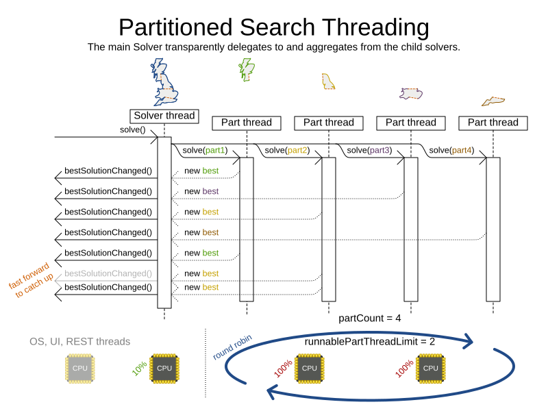
When running a multi-threaded solver, such as Partitioned Search, CPU power can quickly become a scarce resource, which can cause other processes or threads to hang or freeze. However, Timefold Solver has a system to prevent CPU starving of other processes (such as an SSH connection in production or your IDE in development) or other threads (such as the servlet threads that handle REST requests).

As explained in sizing hardware and software, each solver (including each child solver) does no IO during solve() and therefore saturates one CPU core completely. In Partitioned Search, every partition always has its own thread, called a part thread. It is impossible for two partitions to share a thread, because of asynchronous termination: the second thread would never run. Every part thread will try to consume one CPU core entirely, so if there are more partitions than CPU cores, this will probably hang the system. Thread.setPriority() is often too weak to solve this hogging problem, so another approach is used.

The runnablePartThreadLimit parameter specifies how many part threads are runnable at the same time. The other part threads will temporarily block and therefore will not consume any CPU power. This parameter basically specifies how many CPU cores are donated to Timefold Solver. All part threads share the CPU cores in a round-robin manner to consume (more or less) the same number of CPU cycles:

The following runnablePartThreadLimit options are supported:

UNLIMITED: Allow Timefold Solver to occupy all CPU cores, do not avoid hogging. Useful if a no hogging CPU policy is configured on the OS level.
AUTO (default): Let Timefold Solver decide how many CPU cores to occupy. This formula is based on experience. It does not hog all CPU cores on a multi-core machine.
Static number: The number of CPU cores to consume. For example:
```
<runnablePartThreadLimit>2</runnablePartThreadLimit>
```

If the runnablePartThreadLimit is equal to or higher than the number of available processors, the host is likely to hang or freeze, unless there is an OS specific policy in place to avoid Timefold Solver from hogging all the CPU processors.

1.3. Custom thread factory (WildFly, GAE, …)

The threadFactoryClass allows to plug in a custom ThreadFactory for environments where arbitrary thread creation should be avoided, such as most application servers (including WildFly) or Google App Engine.

Configure the ThreadFactory on the solver to create the move threads and the Partition Search threads with it:

<solver xmlns="https://timefold.ai/xsd/solver" xmlns:xsi="http://www.w3.org/2001/XMLSchema-instance"
    xsi:schemaLocation="https://timefold.ai/xsd/solver https://timefold.ai/xsd/solver/solver.xsd">
  <threadFactoryClass>...MyAppServerThreadFactory</threadFactoryClass>
  ...
</solver>