Time patterns
Dealing with time and dates in planning problems may be problematic because it is dependent on the needs of your use case.
There are several representations of timestamps, dates, durations and periods in Java and Kotlin. Choose the right representation type for your use case:
-
DayOfWeekwith or withoutLocalTimeif no date is involved. -
LocalDateif no time is involved. -
LocalDateTimeif your model only works in a single timezone without DST (Daylight Saving Time). -
OffsetDateTimeif your model supports timezones or DST (Daylight Saving Time).-
Avoid
ZonedDateTime, it is error-prone.
-
-
Never use
java.util.Date: it is a slow, error-prone way to represent timestamps.
There are also several designs for assigning a planning entity to a starting time (or date):
-
If the starting time is fixed beforehand, it is not a planning variable (in that solver).
-
For example: in Bed Allocation Scheduling, the arrival day of each patient is fixed beforehand.
-
This is common in multi-stage planning, when the starting time has been decided already in an earlier planning stage.
-
-
If the starting time is not fixed, it is a planning variable (genuine or shadow).
-
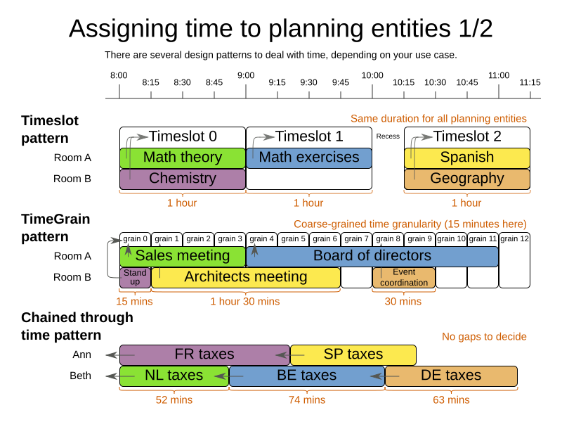
If all planning entities have the same duration, use the Timeslot pattern.
-
For example, in school timetabling, all lectures take one hour. Therefore, each timeslot is one hour.
-
Even if the planning entities have different durations, but the same duration per type, it’s often appropriate.
-
For example, in conference scheduling, breakout talks take one hour and lab talks take 2 hours. But there’s an enumeration of the timeslots and each timeslot only accepts one talk type.
-
-
-
If the duration differs and time is rounded to a specific time granularity (for example 5 minutes) use the TimeGrain pattern.
-
If the duration differs and one task starts immediately after the previous task (assigned to the same executor) finishes, use the Chained Through Time pattern.
-
For example, in time windowed vehicle routing, each vehicle departs immediately to the next customer when the delivery for the previous customer finishes.
-
Even if the next task does not always start immediately, but the gap is deterministic, it applies.
-
For example, in vehicle routing, each driver departs immediately to the next customer, unless it’s the first departure after noon, in which case there’s first a 1 hour lunch.
-
-
-
If the employees need to decide the order of theirs tasks per day, week or SCRUM sprint themselves, use the Time Bucket pattern.
-
For example, in elevator maintenance scheduling, a mechanic gets up to 40 hours worth of tasks per week, but there’s no point in ordering them within 1 week because there’s likely to be disruption from entrapments or other elevator outages.
-
-
Choose the right pattern depending on the use case:
1. Timeslot pattern: assign to a fixed-length timeslot
If all planning entities have the same duration (or can be inflated to the same duration), the Timeslot pattern is useful. The planning entities are assigned to a timeslot rather than time. For example, in school timetabling, all lectures take one hour.
The timeslots can start at any time. For example, the timeslots start at 8:00, 9:00, 10:15 (after a 15-minute break), 11:15, … They can even overlap, but that is unusual.
It is also usable if all planning entities can be inflated to the same duration. For example, in Examination Timetabling, some exams take 90 minutes and others 120 minutes, but all timeslots are 120 minutes. When an exam of 90 minutes is assigned to a timeslot, for the remaining 30 minutes, its seats are occupied too and cannot be used by another exam.
Usually there is a second planning variable, for example the room. In course timetabling, two lectures are in conflict if they share the same room at the same timeslot. However, in exam timetabling, that is allowed, if there is enough seating capacity in the room (although mixed exam durations in the same room do inflict a soft score penalty).
2. TimeGrain pattern: assign to a starting TimeGrain
Assigning humans to start a meeting at four seconds after 9 o’clock is pointless because most human activities have a time granularity of five minutes or 15 minutes. Therefore it is not necessary to allow a planning entity to be assigned subsecond, second or even one minute accuracy. A granularity of 15 minutes, 1 hour or 1 day accuracy suffices for most use cases. The TimeGrain pattern models such time accuracy by partitioning time as time grains. For example, in Meeting Scheduling, all meetings start/end in hour, half hour, or 15-minute intervals before or after each hour, therefore the optimal settings for time grains is 15 minutes.
Each planning entity is assigned to a start time grain. The end time grain is calculated by adding the duration in grains to the starting time grain. Overlap of two entities is determined by comparing their start and end time grains.
The TimeGrain pattern doesn’t scale well. Especially with a finer time granularity (such as 1 minute) and a long planning window, the value range (and therefore the search space) is too big to scale well. It’s recommended to use a coarse time granularity (such as 1 week, 1 day, 1 half day, …) or shorten the planning window size to scale. To resolve scaling issues, the Time Bucket pattern is often a good alternative.
3. Chained through time pattern: assign in a chain that determines starting time
If a person or a machine continuously works on one task at a time in sequence, which means starting a task when the previous is finished (or with a deterministic delay), the Chained Through Time pattern is useful. For example, in Vehicle routing with time windows, a vehicle drives from customer to customer (thus it handles one customer at a time).
The focus in this pattern is on deciding the order of a set of elements instead of assigning them to a specific date and time. However, the time coordinate of each element can be deduced from its position in the sequence. If the elements' position on time axis affects the score, use a shadow variable to calculate the time.
This pattern is implemented using the planning list variable. The planning entity determines the starting time of the first element in its planning list variable. The second element’s starting time is calculated based on the starting time and duration of the first element. For example, in task assignment, Beth (the entity) starts working at 8:00, thus her first task starts at 8:00. It lasts 52 minutes, therefore her second task starts at 8:52. The starting time of an element is usually a shadow variable.
3.1. Chained through time pattern: creating gaps
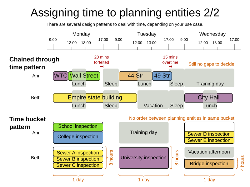
Between planning entities, there are three ways to create gaps:
-
No gaps: This is common when the anchor is a machine. For example, a build server always starts the next job when the previous finishes, without a break.
-
Only deterministic gaps: This is common for humans. For example, any task that crosses the 10:00 barrier gets an extra 15 minutes duration so the human can take a break.
-
A deterministic gap can be subjected to complex business logic. For example, a cross-continent truck driver needs to rest 15 minutes after two hours of driving (which may also occur during loading or unloading time at a customer location) and also needs to rest 10 hours after 14 hours of work.
-
-
Planning variable gaps: This is uncommon, because that extra planning variable reduces efficiency and scalability, (besides impacting the search space too).
3.2. Chained through time: automatic collapse
In some use case there is an overhead time for certain tasks, which can be shared by multiple tasks, if those are consecutively scheduled. Basically, the solver receives a discount if it combines those tasks.
For example when delivering pizza to two different customers, a food delivery service combines both deliveries into a single trip, if those two customers ordered from the same restaurant around the same time and live in the same part of the city.
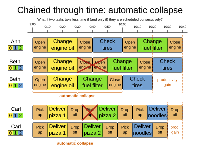
Implement the automatic collapse in the shadow variables that calculate the start and end times of each task.
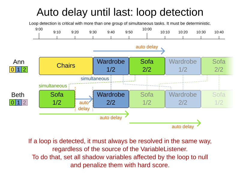
3.3. Chained through time: automatic delay until last
Some tasks require more than one person to execute. In such cases, both employees need to be there at the same time, before the work can start.
For example when assembling furniture, assembling a bed is a two-person job.
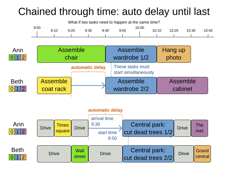
Implement the automatic delay in the shadow variables that calculates the arrival, start and end times of each task. Separate the arrival time from the start time. Additionally, add loop detection to avoid an infinite loop:
4. Time bucket pattern: assign to a capacitated bucket per time period
In this pattern, the time of each employee is divided into buckets. For example 1 bucket per week. Each bucket has a capacity, depending on the FTE (Full Time Equivalent), holidays and the approved vacation of the employee. For example, a bucket usually has 40 hours for a full time employee and 20 hours for a half time employee but only 8 hours on a specific week if the employee takes vacation the rest of that week.
Each task is assigned to a bucket, which determines the employee and the coarse-grained time period for working on it. The tasks within one bucket are not ordered: it’s up to the employee to decide the order. This gives the employee more autonomy, but makes it harder to do certain optimization, such as minimize travel time between task locations.